


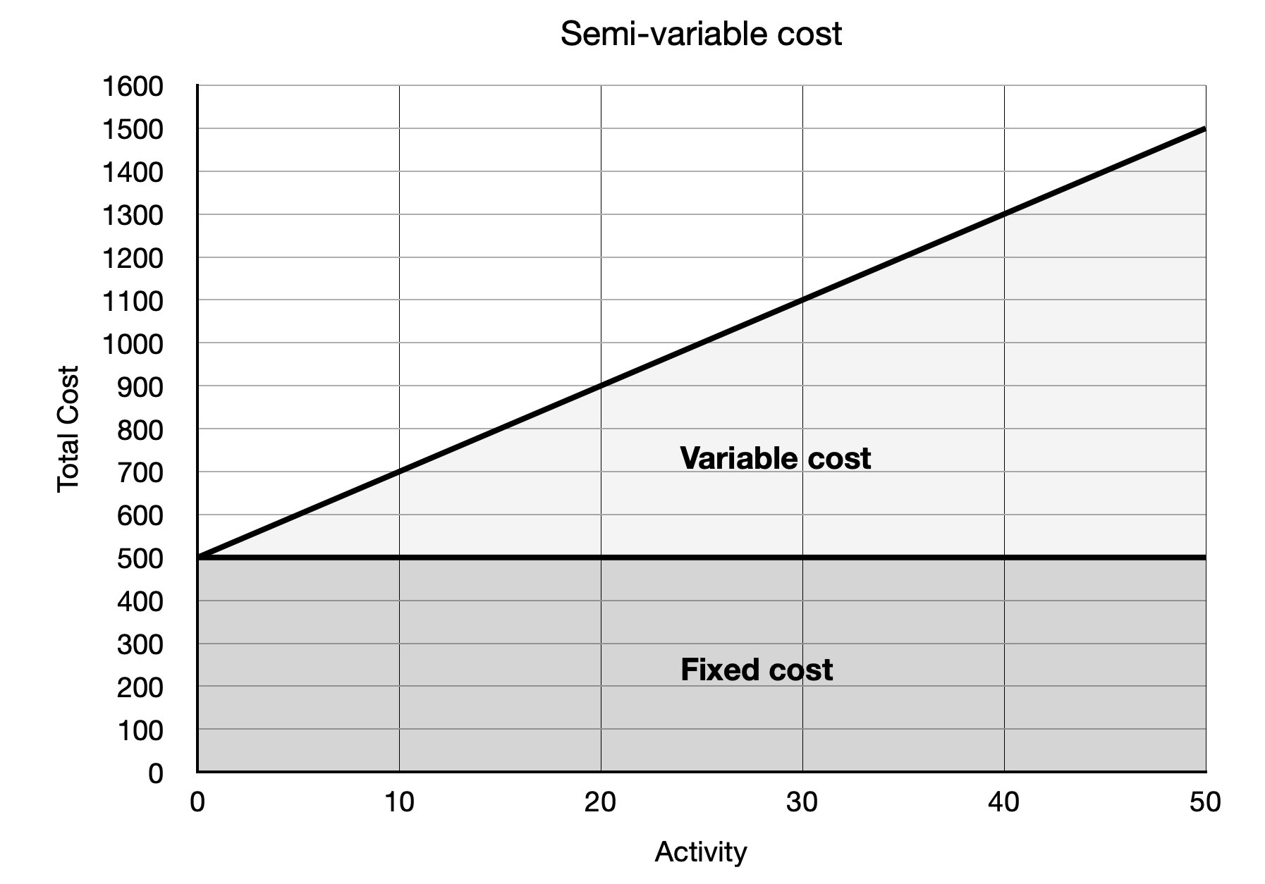
In this example, the fixed cost is already provided, but should it not be, we would need to separate out the fixed and variable costs using one of the methods mentioned below.
The high-low method
This method uses the difference between the costs associated with the highest and lowest activity levels divided by the difference between those activity levels.
It is important to note that extreme distribution of values may yield inaccurate results because outliers are being used to make estimations. The scatter plot can help visualise data points to check for outliers, and if there are few outliers, they could be removed.
The high-low formula
\( \text{Variable Cost} = \frac{\text{Cost}_{high} – \text{Cost}_{low}}{\text{Activity}_{high} – \text{Activity}_{low}} \)
Scatterplot
When we have data points for a dependent and independent variable over time, and the variable pair is measured at the same time at different intervals, we can create a graphical representation to see if any relationship might exist between the two variables.
Regression analysis
Regression analysis uses computation to arrive at the scatterplot’s line of best fit.
The equation of a straight line is:
\( y = a + bx \)
Where:
- y is the dependent variable
- x is the independent variable
- a is the intercept
- b is the gradient
To calculate the gradient line we have to first solve for b using the least squares method.
\( b = \frac{n\sum xy – (\sum x)(\sum y)}{n\sum x^2 – (\sum x)^2} \)
To calculate b by hand with pen, paper and a calculator, we need to solve for all the values and then plug them into the formula.
- ∑x
- ∑y
- ∑X²
- ∑xy
- ȳ
- x̄
To calculate a, we use the formula
\( a = y – bx \)
Once we have calculated the slope and intercept values, we can predict y for any given value of x.
Correlation
R tells us the strength and direction of the relationship
R-squared tells us how much of the variation – what percentage – is explained by the model.
The formula for r is:
\( r = \frac{n\sum xy – (\sum x)(\sum y)}{\sqrt{[n\sum x^2 – (\sum x)^2][n\sum y^2 – (\sum y)^2]}} \)
We need to plug the following values into the formula to get to r.
- ∑x
- ∑y
- ∑X²
- ∑y²
- ∑xy
